Introduction to SciPy

Introduction to SciPy#

What is SciPy?#

SciPy (Scientific Python) is a Python library used for scientific and technical computing. It is a collection of mathematical algorithms and convenience functions built on the NumPy library.

The SciPy package contains various sub-packages that are dedicated to common issues in scientific computing. See the table below:

Subpackage	Description
cluster	Clustering algorithms
constants	Physical and mathematical constants
fftpack	Fast Fourier Transform routines
integrate	Integration and ordinary differential equation solvers
interpolate	Interpolation and smoothing splines
io	Input and Output
linalg	Linear algebra
ndimage	N-dimensional image processing
odr	Orthogonal distance regression
optimize	Optimization and root-finding routines
signal	Signal processing
sparse	Sparse matrices and associated routines
spatial	Spatial data structures and algorithms
special	Special functions
stats	Statistical distributions and functions

In this tutorial, we will briefly introduce interpolate and stats subpackages.

Install SciPy#

Install SciPy using pip

Run the following command in the terminal:

pip install scipy
Install SciPy using Anaconda

conda install -c anaconda scipy

Interpolation#

SciPy provides functions to perform interpolation. Here’s an example of 1D interpolation using scipy.interpolate.interp1d():

import numpy as np
from scipy.interpolate import interp1d
from matplotlib import pyplot as plt

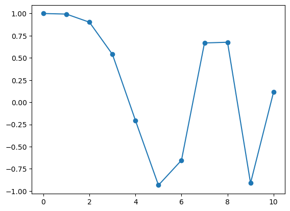
We first generate a test dataset x and y below:

x = np.linspace(0, 10, num=11, endpoint=True)
y = np.cos(-x**2/9)
plt.scatter(x, y)

<matplotlib.collections.PathCollection at 0x1226aae00>

../_images/8216f4cc53bc07b009ae783455e8c448a5a039bcf41d20120bcd3fef66c5ab61.png

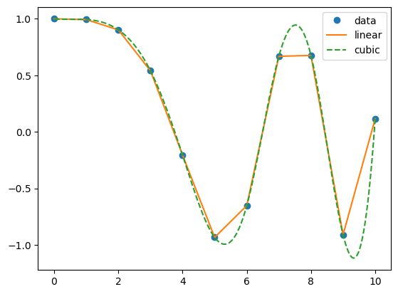
Then we can try to find out the values in between the points using interpolation function interp1d(). The default method is linear interpolation if you do not specify.

f = interp1d(x, y)  # the default is linear interpolation
xnew = np.linspace(0, 10, 1000)
ynew = f(xnew)   # use interpolation function returned by `interp1d`

# Plot the results
plt.plot(xnew, ynew)
plt.scatter(x,y)
plt.show()

../_images/6be7deedffe72c97c91d30058a85e0891c728df47f3e657fbf8c155f29a2cdb7.png

We can also try other interpolation method such as “cubic” using kind="cubic"

f2 = interp1d(x, y, kind='cubic')

# Plot the results
ynew2 = f2(xnew)   # use interpolation function returned by `interp1d`
plt.plot(x,y,'o',xnew,ynew,'-',xnew,ynew2,'--')
plt.legend(['data', 'linear', 'cubic'], loc='best')
plt.show()

../_images/a219660d7b6b2f53c7964f02e96840fe4f91d8ddd5e2cf9583c218a61c4ef375.png

Methods that you can choose from interp1d include the followings. Feel free to try out yourself.

Linear
Nearest
Zero
S-linear
Quadratic
Cubic

Exercise in Interpolation#

Time: 5 minutes

Can you generate a new dataset and try out different interpolation methods using interp1d or other functions.

Check more details in the official website.

Statistics#

The stat subpackage is very useful for statistic usage. Here we will introduce the example of linear regression.

We will import the stats first:

from scipy import stats

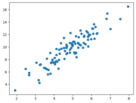
Generate the data:

# Generate some data for linear regression
x = np.random.randn(100) + 5 # A random sample of 1000 numbers from a normal (Gaussian) distribution with mean 5
y = 2*x + np.random.randn(100) # A random sample of 1000 numbers from a normal (Gaussian) distribution with mean 0
plt.scatter(x,y)

<matplotlib.collections.PathCollection at 0x127e2b7f0>

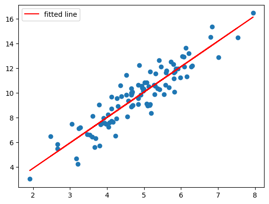
../_images/4a86f88e0cbac11b45c588f4081b183c8fa4805766e47dc631d539276607a4c5.png

# Perform a linear regression
slope, intercept, r_value, p_value, std_err = stats.linregress(x,y)
print(f'slope = {slope}, intercept = {intercept}, p_value = {p_value}')
print(f'r_value = {r_value}, std_err = {std_err}')

slope = 2.060071419651353, intercept = -0.22220682062170027, p_value = 1.2214866625946454e-40
r_value = 0.9159285637898558, std_err = 0.09118460593222329

# Plot the results
plt.scatter(x,y)
plt.plot(x, intercept + slope*x, 'r', label='fitted line')
plt.legend()
plt.show()

../_images/0d808d4b32324656c42c67fb2569a503abb72eb5ae807c7cbf9c5abfea3d1c3a.png